From the Baltic Sea to South Africa: AIS data for Baltic Scope

Slide 1 of 17: From the Baltic Sea to South Africa AIS data for Baltic Scope Manuel Frias HELCOM Secretariat Baltic Scope partner meeting Szczecin, Poland June 2016

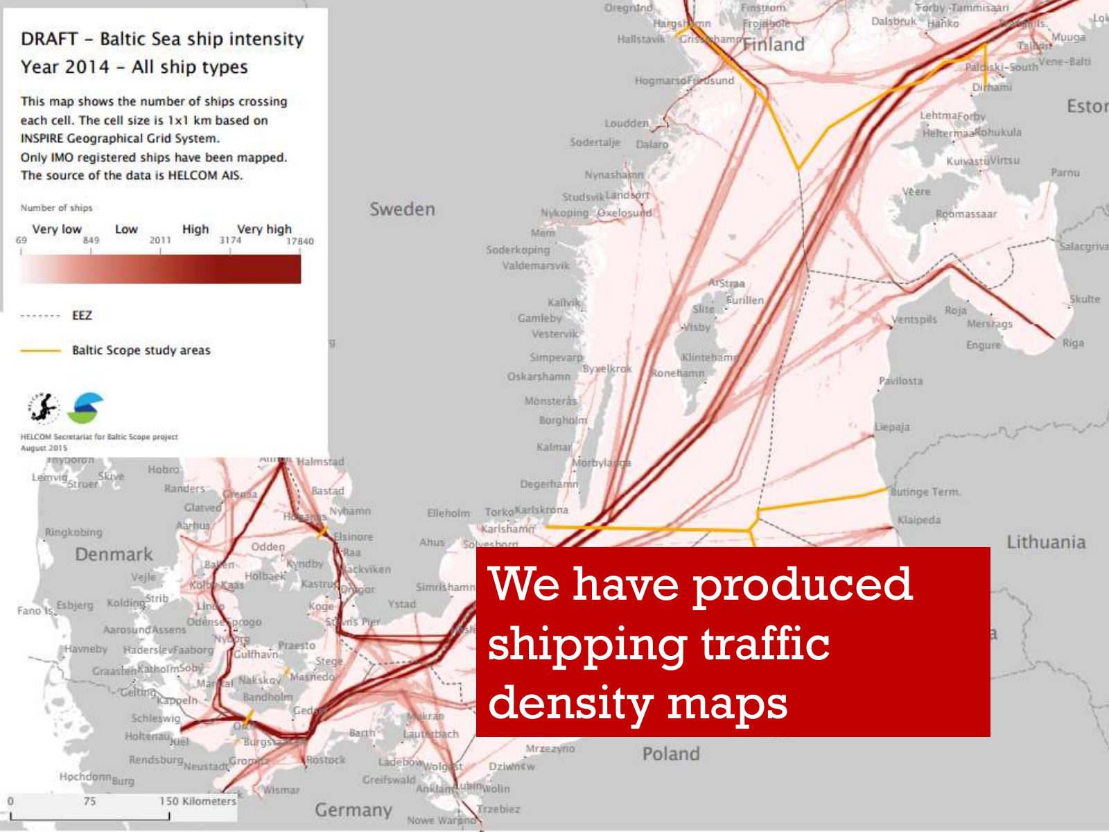
Slide 2 of 17: We have produced shipping traffic density maps

Slide 3 of 17: What is a density map?

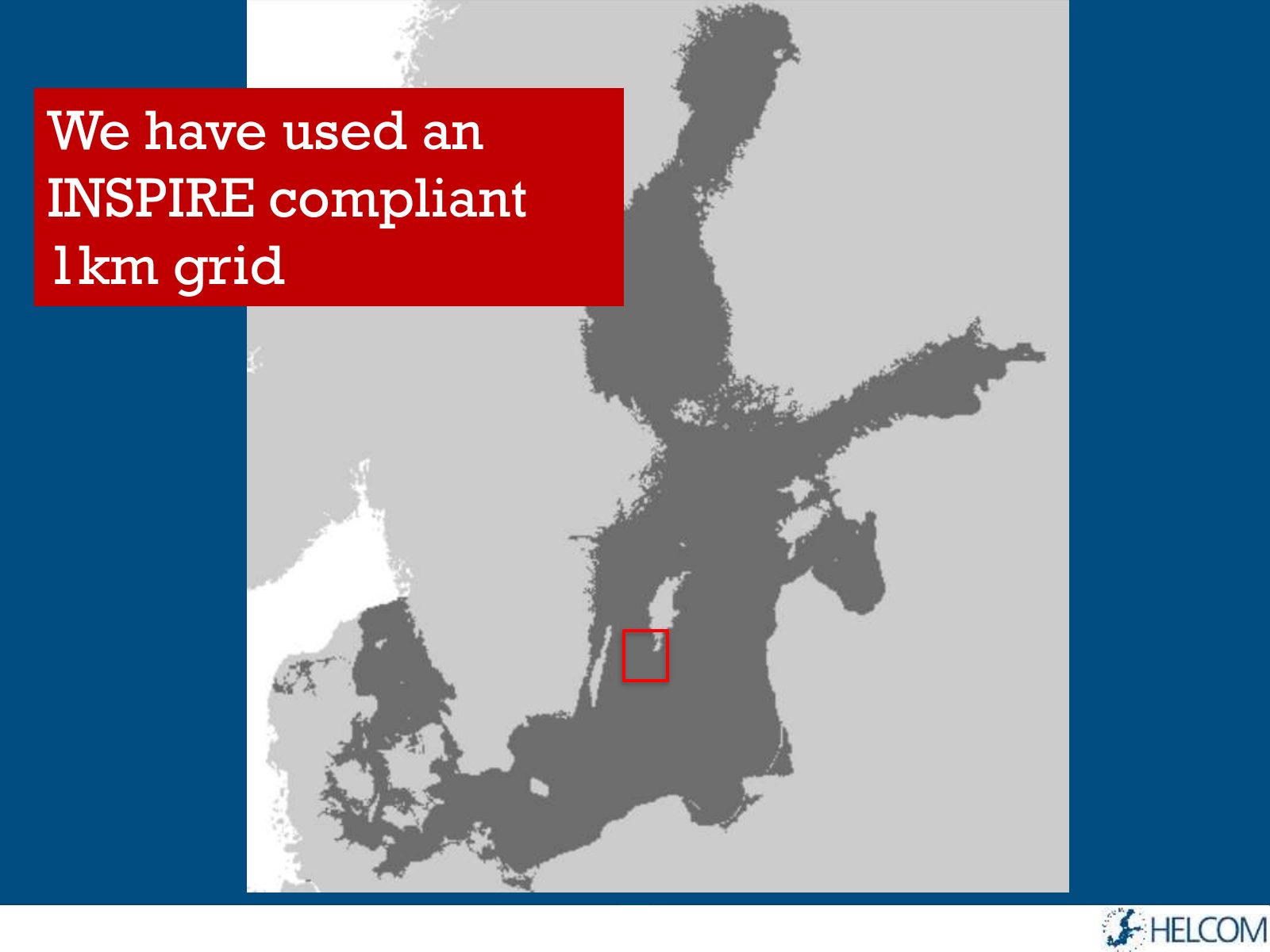
Slide 4 of 17: We have used an INSPIRE compliant 1km grid

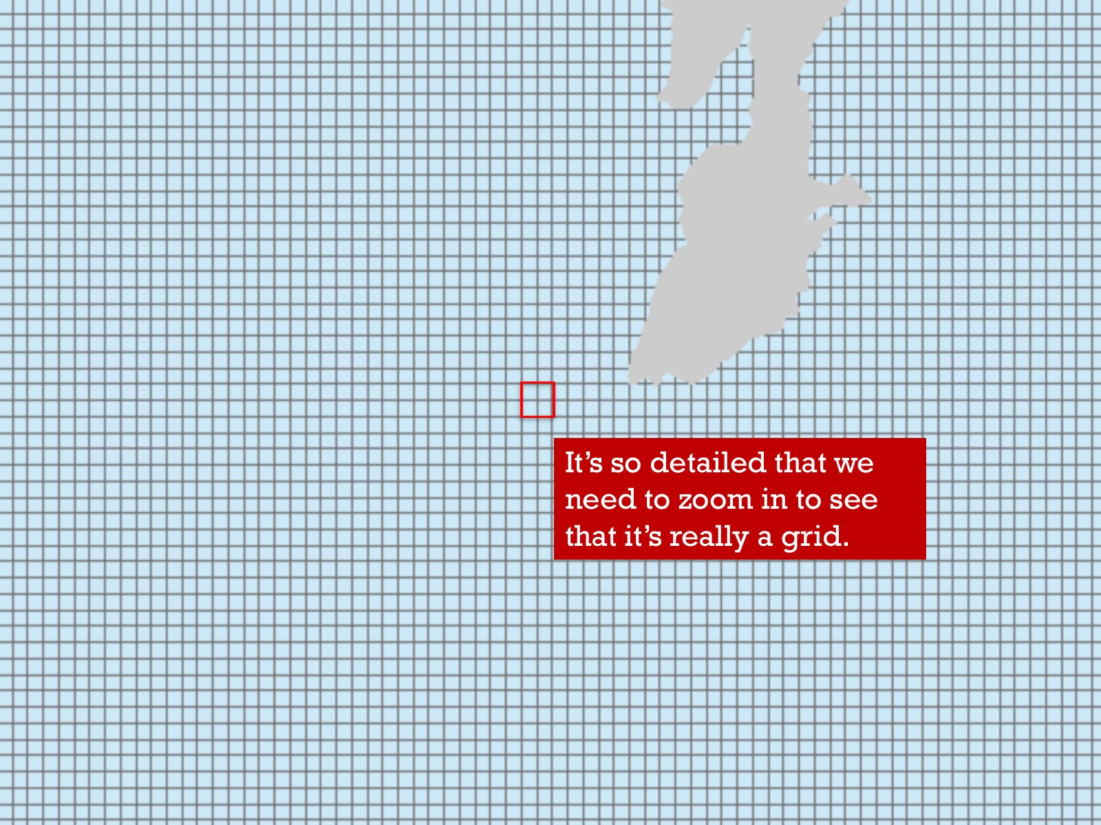
Slide 5 of 17: It’s so detailed that we need to zoom in to see that it’s really a grid.

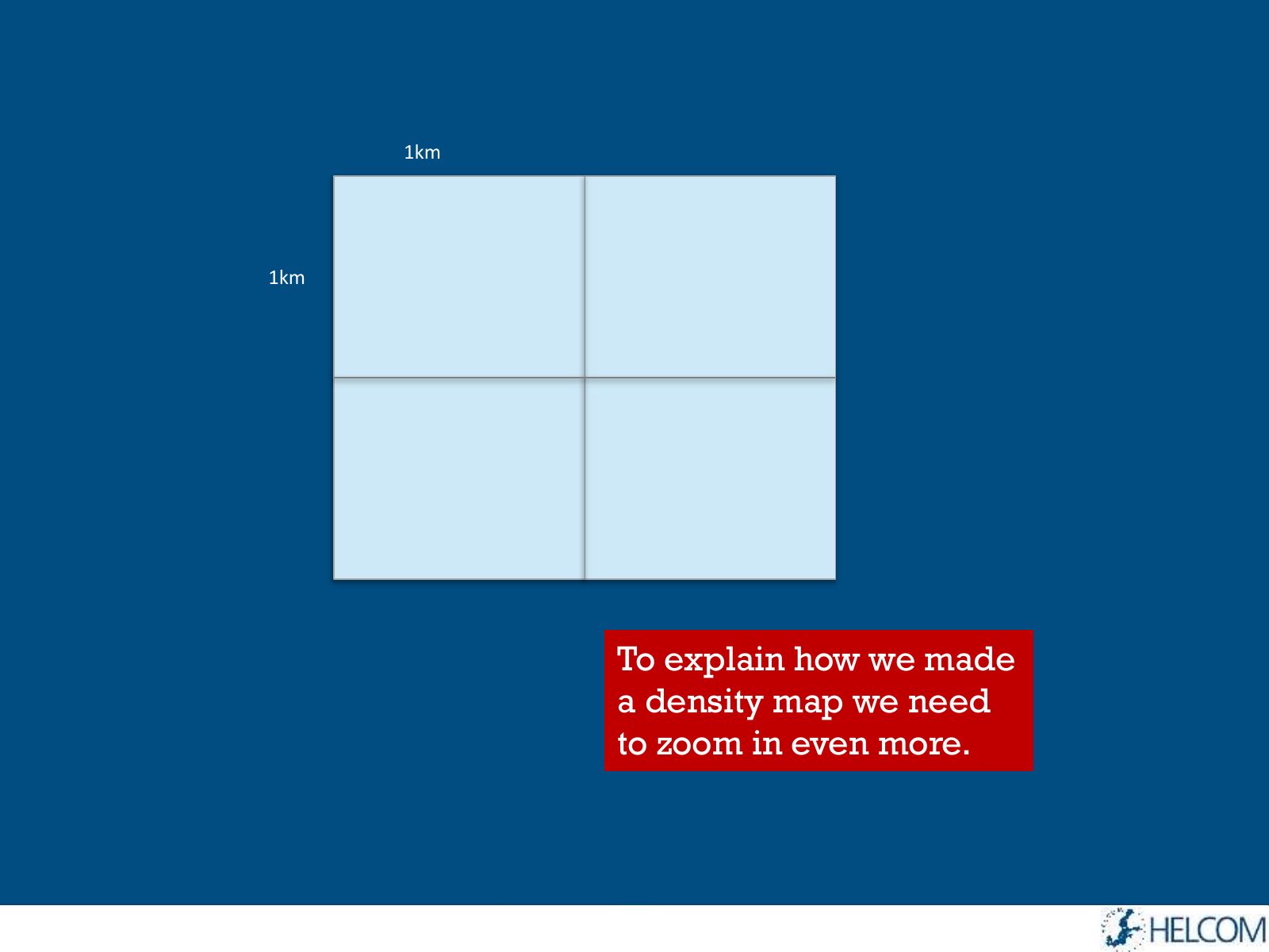
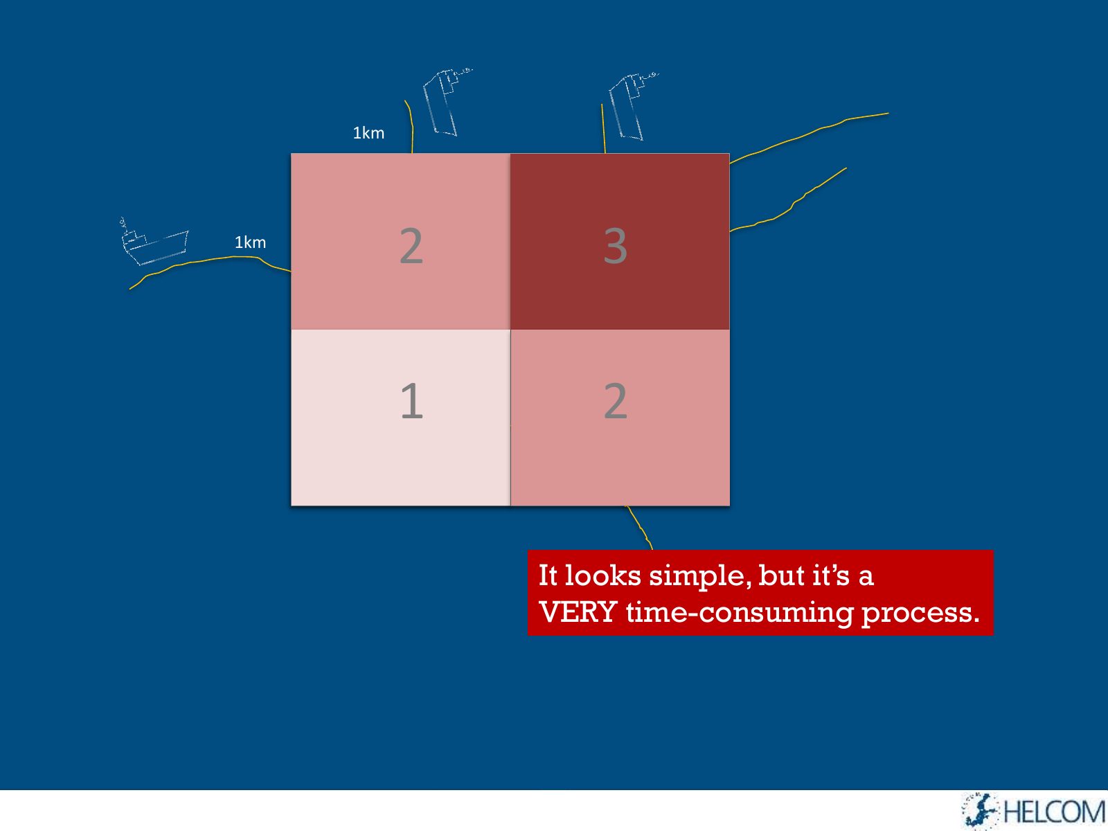
Slide 6 of 17: 1km 1km To explain how we made a density map we need to zoom in even more.

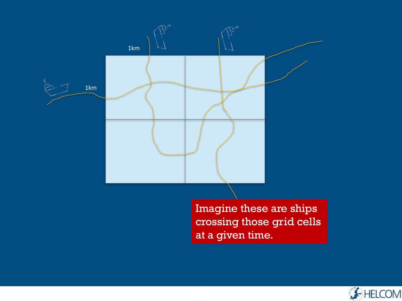
Slide 7 of 17: 1km 1km Imagine these are ships crossing those grid cells at a given time.

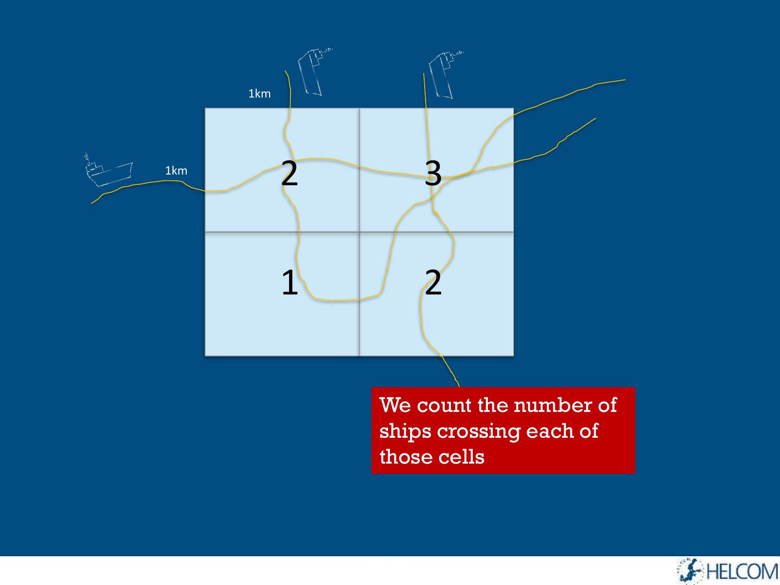
Slide 8 of 17: 1km 1km 2 3 1 2 We count the number of ships crossing each of those cells

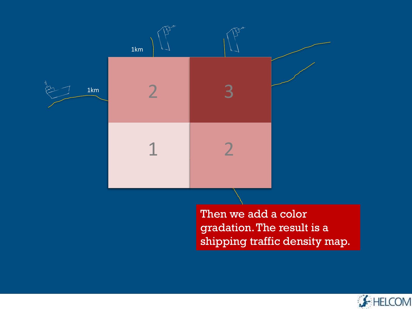
Slide 9 of 17: 1km 1km 2 3 1 2 Then we add a color gradation. The result is a shipping traffic density map.

Slide 10 of 17: 1km 1km 2 3 1 2 It looks simple, but it’s a VERY time-consuming process.

Slide 11 of 17: How big is one year of AIS data?

Slide 12 of 17: 2013 contains 1,3 BILLION rows

Slide 13 of 17: If we printed them we would need 30 MILLION A4 pages

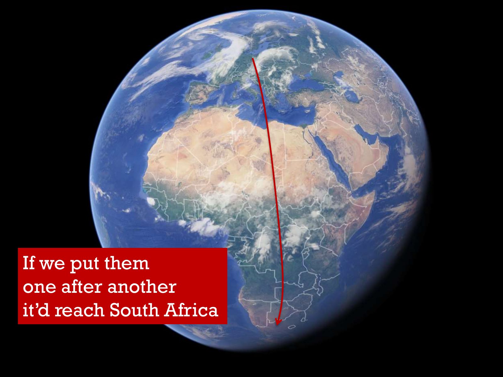
Slide 14 of 17: If we put them one after another it’d reach South Africa

Slide 15 of 17: We have provided maps… 13 2014 Cargo Tanker Passenger Fishing

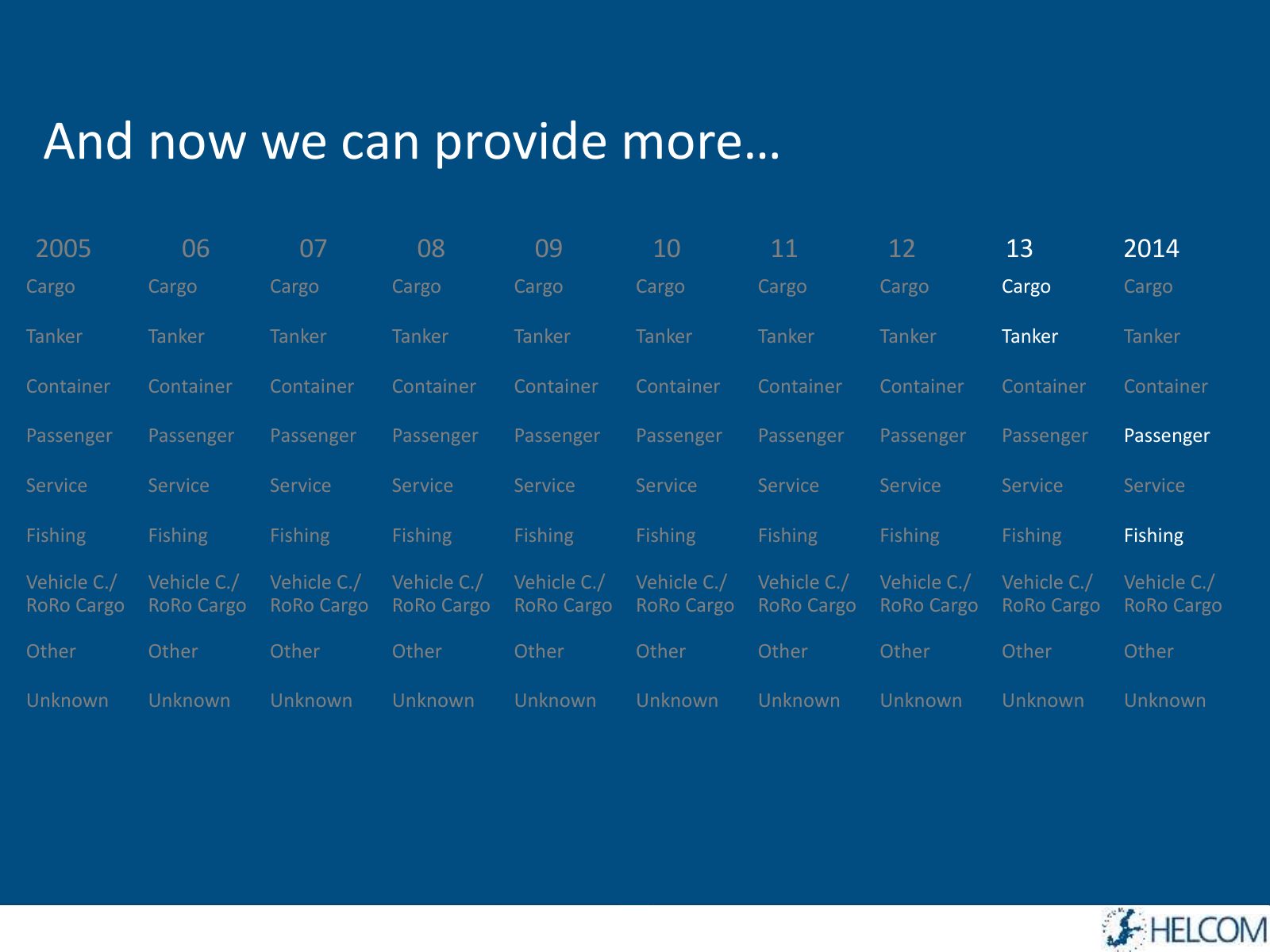
Slide 16 of 17: And now we can provide more… 2005 06 07 08 09 10 11 12 13 2014 Cargo Cargo Cargo Cargo Cargo Cargo Cargo Cargo Cargo Cargo Tanker Tanker Tanker Tanker Tanker…

Slide 17 of 17: So if you want more just tell us!